Spatial Analysis

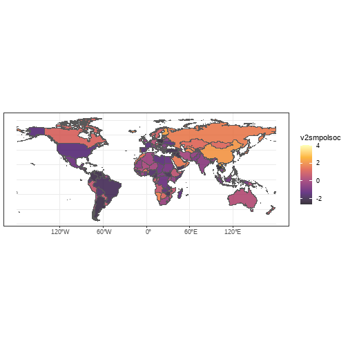
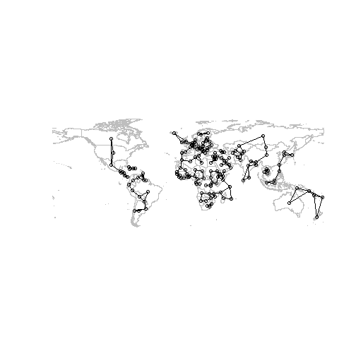
# Spatial Analysis
## A Short Introduction
### Semuhi Sinanoglu
### University of Toronto
### 2021-03-05

---

---
class: inverse, center, middle
background-image: url("introspatial.jpg")
background-position: center
background-size: contain

---

# Presentation Outline

- What do we mean by spatial data?

- What the heck is spatial dependence?

- Why should we take it seriously?

- When should we apply spatial analysis?

- Which R packages and skills required?

- Two main approaches to spatial analysis

- A basic R application

- Additional Resources

- Extra: Spatial Non-stationarity; Spatial Analysis for Panel Data

---

---

# Spatial data

- areal data

--
---

# Spatial data

- point pattern data

- space doesn't always mean geography

---

---

# Spatial Dependence

--
.pull-left[
**1. Diffusion**
]

.pull-right[
There are plenty of applications in PoliSci: 
- diffusion among IOs (Sommerer and Tallberg 2018)
- coups (Miller et al. 2016)
- conflict (Kelling and Lin 2019)
- protests (Crabtree et al. 2015)
- self-determination (Cunningham and Sawyer 2017)
]

**2. Attributional Dependence**

**3. Spatially Correlated Exogenous Shocks**

---

---

# Spatial Dependence

A generic spatial model for cross-sectional data from `$Anselin(1988, 34)$`:

`$$y= \rho W_{1} y + X\beta + \epsilon$$`

`$$\epsilon = \lambda W_{2}\epsilon + \mu$$`
--

- What if diffusion process exists?

+ Omitted variable bias

+ OLS assumption violation

- What if error terms are clustered?

--
  + OLS assumption violation

- Generic example: the impact of development on democracy

---

---

# Spatial Analysis

If the response variable is spatially dependent? Nope.

---

# Spatial Analysis

If the primary interest is not spatial inference, then there might be other estimation strategies instead of spatial analysis.

- Let's say there is no diffusion but just error dependence. Can we just use clustered standard errors? You may use `cluster.vcov` function from `multiwayvcov` or `sandwich` packages. When would this work?
--

- How about HAC-estimators? `vcovHAC()` from `sandwich` package.

- Then check `lm.morantest()` from `spdep` package.<sup>1</sup>

.footnote[
  The global Moran's I measure can only help us to identify whether there are any clustering characteristics in a given space, but cannot delineate clustering regions. To that aim, you need local Moran's I (LISA) statistic. 
  
  For a **very interesting** paper on using spatial analysis and LISA statistic for mixed-method case selection strategy, see **Ingram and Harbers, 2019, "Spatial Tools for Case Selection: Using LISA Statistics to Design Mixed-Methods Research", PSRM.**]

---

---

## Mapping skills

.pull-left[
- First, you should be able to import spatial data into R. 
  + `rnaturalearthdata` and `rnaturalearth` packages help you access free vector and raster map data from the Natural Earth. 
]

.pull-right[
<div class="figure" style="text-align: right">
<img src="vector.PNG" alt="Vector vs. raster data. Source: ESRI." width="70%" height="70%" />
<p class="caption">Vector vs. raster data. Source: ESRI.</p>
</div>
]

+ Spatial data are stored in different formats, and sometimes it is painful to quickly import it to R environment. Two packages are helpful: `readOGR` function from `rgdal` package, or `raster` package.
  
--

+ `sp` package has been replaced by `sf`. Get familiar with the `sf` package. Instead of relying on ESRI shapefiles, `sf` package allows storing spatial data with simple feature attributes such as y point, line, and polygon geometries. What makes it beautiful is that it is compatible with tidyverse and allows us to treat spatial data object as data.frames. You may use `geom_sf()` function to draw incredible maps.

---
## Spatial Analysis

.pull-left[
  + You need to know how to calculate a weighting contiguity matrix. `spdep` package.
  
  + For spatial estimation: `spatialreg` package.
]

.pull-right[
  How do we define neighbors? Queen contiguity, k-nearest neighbor etc.
  
<div class="figure" style="text-align: right">
<img src="contiguity.jpg" alt="Source: Angela Li, Spatial Analysis Workshop." width="1280" />
<p class="caption">Source: Angela Li, Spatial Analysis Workshop.</p>
</div>

]

---
class: inverse, center, middle
# Two Approaches to Spatial Estimation
---
# Spatial Estimation

`$$y= \rho W_{1} y + X\beta + \epsilon$$`

`$$\epsilon = \lambda W_{2}\epsilon + \mu$$`

- Spatial error model

- Spatially lagged model

---
class: inverse, center, middle
# A Basic R Application

Is polarization contagious?

---
<img src="realworlddata.jpg" width="100%" height="100%" />
---

## Installing Packages and Data Setup

```r
## Packages ----------------------
packages <- c("spdep", "spatialreg", "sf", "here",
          "rnaturalearth", "rnaturalearthdata", "tidyverse")
installed <- packages %in% rownames(installed.packages())
if (any(installed == FALSE)) install.packages(packages[!installed])
invisible(lapply(packages, library, character.only = TRUE))

## Data Setup --------------------
set.seed(123)
options(scipen = 999)

## V-dem Data
vdem <- readRDS("data/vdem.RDS")
vdem <- vdem %>% filter(year==2018) %>%
  select(country_name, v2smpolsoc, v2cacamps, v2x_delibdem, v2xel_frefair,
         v2x_cspart, v2x_freexp_altinf, v2regsupgroupssize)

## SF Data
*world <- ne_countries(scale = "large", returnclass = "sf",
*                     country = vdem$country_name)
world <- world %>% rename(country_name = sovereignt)
world <- left_join(world, vdem, by="country_name")
```

---
## Visualization

```r
world %>%
  ggplot() + geom_sf(aes(fill=v2smpolsoc)) +
  scale_fill_viridis_c(alpha = .8, option="inferno") + 
  theme_bw()
```

![](slides_files/figure-html/visual-1.png)

---
## Spatial Weights

```r
## Spatial Weight Matrix ---------------
coords <- st_centroid(st_geometry(world), of_largest_polygon=TRUE)
col.knn <- knearneigh(coords, k=2) ## k-nearest approach

nb.matrix <- knn2nb(col.knn)
list.w <- nb2listw(nb.matrix, style = "W")

plot(st_geometry(world), border="grey")
plot(knn2nb(col.knn), coords, add=TRUE)
```

---
## Neighborhood Plot
![](slides_files/figure-html/spatial-1.png)
---
## Spatial Estimation

```r
mod1 <- v2smpolsoc ~ v2x_delibdem + v2xel_frefair +
  v2x_cspart + v2x_freexp_altinf + v2regsupgroupssize

model1 <- lagsarlm(mod1, data = world, listw = list.w) #spatial lag
model2 <- errorsarlm(mod1,data = world, listw = list.w) #spatial error
```
---
## Spatial Lag Model

```
## 
## Call:lagsarlm(formula = mod1, data = world, listw = list.w)
## 
## Residuals:
##        Min         1Q     Median         3Q        Max 
## -2.9249528 -1.0411154  0.0088733  1.0744493  3.7873997 
## 
## Type: lag 
## Coefficients: (asymptotic standard errors) 
##                     Estimate Std. Error z value  Pr(>|z|)
## (Intercept)         0.206181   0.362416  0.5689 0.5694192
## v2x_delibdem        3.254312   1.199808  2.7124 0.0066806
## v2xel_frefair      -0.080468   0.783829 -0.1027 0.9182322
## v2x_cspart          0.712913   1.047820  0.6804 0.4962655
## v2x_freexp_altinf  -3.218073   0.976528 -3.2954 0.0009827
## v2regsupgroupssize  0.133994   0.126836  1.0564 0.2907708
## 
## Rho: 0.0086914, LR test value: 0.010984, p-value: 0.91653
## Asymptotic standard error: 0.081473
##     z-value: 0.10668, p-value: 0.91505
## Wald statistic: 0.01138, p-value: 0.91505
## 
## Log likelihood: -275.7669 for lag model
## ML residual variance (sigma squared): 1.7623, (sigma: 1.3275)
## Number of observations: 162 
## Number of parameters estimated: 8 
## AIC: 567.53, (AIC for lm: 565.54)
## LM test for residual autocorrelation
## test value: 0.028692, p-value: 0.86549
```
---
## Spatial Error Model

```
## 
## Call:errorsarlm(formula = mod1, data = world, listw = list.w)
## 
## Residuals:
##        Min         1Q     Median         3Q        Max 
## -2.9292491 -1.0394330  0.0084675  1.0743215  3.8040223 
## 
## Type: error 
## Coefficients: (asymptotic standard errors) 
##                     Estimate Std. Error z value  Pr(>|z|)
## (Intercept)         0.197768   0.363398  0.5442 0.5862899
## v2x_delibdem        3.253170   1.200105  2.7107 0.0067134
## v2xel_frefair      -0.064444   0.785808 -0.0820 0.9346386
## v2x_cspart          0.712840   1.049018  0.6795 0.4968015
## v2x_freexp_altinf  -3.217813   0.976969 -3.2937 0.0009889
## v2regsupgroupssize  0.132180   0.127106  1.0399 0.2983796
## 
## Lambda: 0.013242, LR test value: 0.021301, p-value: 0.88396
## Asymptotic standard error: 0.084251
##     z-value: 0.15717, p-value: 0.87511
## Wald statistic: 0.024702, p-value: 0.87511
## 
## Log likelihood: -275.7618 for error model
## ML residual variance (sigma squared): 1.7621, (sigma: 1.3275)
## Number of observations: 162 
## Number of parameters estimated: 8 
## AIC: 567.52, (AIC for lm: 565.54)
```
---
class: inverse, center, middle
# Additional Resources
---
# Additional Resources

- Darmofal, David. 2015. Spatial Analysis for the Social Sciences. New York: Cambridge University Press. 
- Ward, Michael, and Kristian Gleditsch. 2011. Spatial Regression Models. New York: SAGE Publications, Inc.
- Chi, Guangqing, and Jun Zhu. 2019. Spatial Regression Models for the Social Sciences. New York: SAGE Publications, Inc.
]

- https://rspatial.org/

## People to Follow

- Robert J. Franzese 
- Matthew Ingram
]

---
class: inverse, center, middle
# Thanks!
---

# Extra: Spatial Non-stationarity

In order to explore spatial heterogeneity, one data-driven technique that may be used is Geographically Weighted Regression.

Local regression with kernel smoothing:

`$$y_{i} = m(x_{i}) + \mu_{i}$$`
<img src="kernel.jpg" width="60%" height="60%" style="display: block; margin: auto;" />

To run GWR with adaptive kernel, you can use `gwr.sel` function from `spgwr` package.